A Kafkaesque experience…

Following this John, Phil and Ciaran went for another acclimatization trip, this time up to a col at 4,700m (photo below).

Ciaran on our acclimatization trip.

But there was still no sign of Robert…  We were supposed to have met him at Osh off his flight from Moscow.

Meanwhile, back in Osh, Robert was tearing his hair out trying to find what had happened to a holdall full of climbing kit; most of his worldly possessions. Here, in his own words, is an account of what happened.

I left ship in Aberdeen harbour, jumped in my car and made for Edinburgh. I spent the night there then caught a train the next morning, arriving at Heathrow in plenty of time for my flight.

Especially since my flight was delayed by two hours.

Thus I found myself in Dusseldorf, being re-routed back to London! I was assured my luggage would follow me and everything would be fine. I was bounced back to London, trying to ignore the feeling of dread in my stomach; what would go wrong next? I flew London-Moscow DME and spent the least enjoyable 17 hours of my life in that airport, a Kafkaesque experience I have no urge to repeat or to describe further.

I finally landed in Osh (long after Phil, Ciaran and John had departed for Batken), went to the carousel and waited for my holdall. And waited, and waited. Once all the other luggage was gone I trailed despondently to the lost luggage office and filed a report. I was kicked out with only what I had in my hand luggage; one pair of pants, no spare socks and no idea how to get to the hostel. Fortunately Munar, the owner, had come to meet me. It’s a twenty minute drive; I reached my bunk and passed out.

I spent the next five (yes, five) days in Osh trying desperately to find my kit; depending on who I spoke to (S7, BA or Moscow airport staff) it was in London, Moscow or Dusseldorf. All the time I grew more and more stressed, knowing that I was falling further and further behind schedule and that my chances of getting a crack at Muz Tok (or indeed anything) were going from bad to worse.

Finally though I got the bus to the airport to find my holdall sitting in a dusty concrete building, looking very tired and stressed, if a holdall can do that.

I got a taxi to the bus station and found the mashrutka that said ‘BaMp£3kek’ or something like that (Batken) on the front, paid my 300 com (£3) and braced myself for a seven hour rumble across south west Kyrgyzstan.

I arrived at Batken later that day. I had a rough plan from this point; find a taxi driver and ask to be taken to Batken travel services (I had a map showing the way to their base). This very poor plan didn’t have to be put into operation as Zhunusbek, the owner of the company, met me off the bus. We drove straight out of town, after two hours turning off a large, straight road and following a dirt track that soon became a river bed for miles up into the hills. At the end of this, the most improbable road I’ve ever seen, was a hamlet of small huts; Sary-Zhaz.

I spent the night there under a canvas tent with ‘Red Crescent of Iran’ written on it. The next day Talivek, my guide for the next two days, loaded my equipment and bag of watermelons (another huge oversight on my part, I had neglected to bring much other than four watermelons and a carrier bag full of bread) onto two donkeys and beat them with a stick till they started uphill towards base camp. At last!

John has done a good job of describing the walk to basecamp. My experience was slightly different in that I ended up sleeping the night in a shepherds hut with Talivek and two other locals who very kindly shared their meal and gallons of tea with me.

The next day we reached basecamp. Phil, Ciaran and John were elsewhere so I made myself comfortable and bid farewell to Talivek, who headed back down the valley on one of the donkeys with the other trotting after him.

I woke early the next day and crossed the river, wading up to my waist in the glacial meltwater. I slogged up to a col at 4100m to kickstart my acclimatisation. As I made my way down I saw movement at basecamp; the guys were back!

Glacial meltwater streams are at their smallest in the early morning. By late afternoon they are always a lot bigger. The stream I’d barely managed to cross hours earlier as now a raging torrent. I stuck my trainers in my backpack and began wading across. As I reached the halfway point, knowing that it was about to get deeper and finding it at my stomach already it was plain that I was going to be swept off my feet. I took the initiative and launched for the other side, a desperate doggy-paddle to safety, sustaining a cut toe and a bruised knee in the process.

I didn’t want to get my socks bloody so I turned up at basecamp barefoot, bleeding and soaking wet, much to the amusement of my friends (John -‘Haha, exactly how I expected you to arrive’).

Of course, this is a highly condensed version of events; I’ve omitted loads of details that while fascinating to me would be boring to anyone else. In a nutshell though this post brings us up to the point where we are all in base camp and preparing for the first forays towards Muz Tok…

Robert’s donkey.

 

 

The power of the matrix (not the film…)

The idea of exploratory mountaineering can conjure up visions of the Fedchenkos walking up the Jiptik valley and sketching out the locations of the peaks surrounding the Jiptik / Schurovsky glacier, or Shipton and Tilman setting up their plane table in the Nanda Devi sanctuary to survey the remotest corners of British India.  But what does exploration entail when the whole world is at your fingertips on google earth?  Well, the good news (for those who want to explore) is that google earth only gives you a quite limited set of information.  It can give you only the vaguest hint of whether a remote mountain valley is accessible or not – I should know, after my 2014 trip to Kyrgyzstan!  The resolution of the surveying is poor compared to the maps we are used to in Europe from the British Ordnance Survey (OS) or the French Institut Geographique National (IGN), for instance.  And information on the terrain is lacking, it is hard to say if a slope is a pleasant grassy ramble or a terrifying scrabble of dangerous unstable choss.  You cannot see how easy it will be to cross a river, or whether there are seracs, etc, etc.

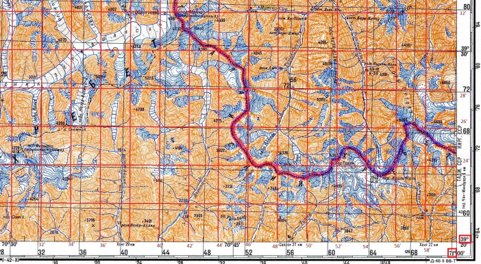
In the former Soviet Union however, there are better maps available than google maps / earth.  The entire USSR was mapped to a high standard during the Soviet era, and at least a large proportion of these maps are now available to download for free from maps.vlasenko.net.  As a subjective opinion, I would say that the surveying on these maps is as good as that on the OS or IGN maps, and the Soviet maps have a certain beauty about them:

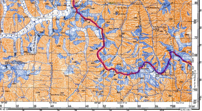
But there are shortcomings; generally they are only available in 1:100,000 resolution – understandable when you consider the size of the country the Soviets had to map!  So the features on display on the maps are quite limited compared to what we are used to on OS or IGN maps and information on the kind of terrain underfoot is sometimes also limited.  The youngest of the Soviet maps were done in circa 1985 and the glaciers have receded a lot since then.  And there is also another problem – the Soviet maps use a datum (Pulkovo 1942 Krasovskii spheroid) which absolutely no-one uses anymore.  Try finding a GPS with that one on!

So a few years ago I developed a method for drawing onto the electronic copy of the Soviet map a WGS84 datum; this is the datum used by google earth and available on any GPS.  The method involved selecting 3 prominent summits or other land marks, obtaining the co-ordinates of their pixels on the electronic copy of the Soviet map and then using google earth to obtain the WGS84 datum longitude and latitude.  Using this information you can then calculate where to put the WGS84 longitude and latitude grid lines (i.e. the datum) on the map – even accounting for the fact that the grid lines do not run parallel to the x and y axes.

So you can now turn on your GPS, read off your location and place yourself on the map.  So when your driver tells you that you have arrived at the point he agreed to drop you off you can inform him that there is another 10 miles still to go,  when you are jungle-bashing your way up some remote valley you can see what a depressingly short distance you have advanced in the past 4 hours, etc. etc.  You can see the reasons why doing this is worth the effort!

My previous method, however, had the shortcoming that, whilst you can use the co-ordinates of some additional summits or landmarks to check that your grid lines are not too wide of the mark, you can only directly use 3 data points in calculating where they should be.  And in each data point there must be some error – google earth often chops the tops off summits and consequently can get them in the wrong location, stream and road junctions can move a bit, etc.  Here is an example of a data point:

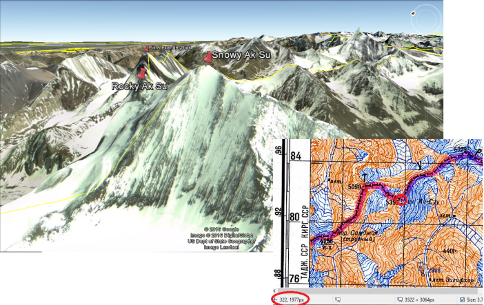
The summit of Ak Su is on the same Soviet map as the Jiptik valley so was used as one of the data points for the calibration.  Snowy Ak Su is the higher and more pronounced summit, which has a placemark on the Soviet map.  You read off the pixels from the map, and the WGS84 latitude and longitude from the google earth placemark.

So this spring I developed a more accurate method which allows you to use as many data points as you have the patience to enter, and use regression analysis to work out the locations for the grid lines which will produce the smallest error in the conversion between pixels and WGS84 co-ordinates for all the data points you have entered.

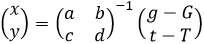
The method involves some simple use of matrices.  You begin by representing the transition between the co-ordinates of the pixels of a given location on the map (x and y) and the longitude and latitude (g and t) using a matrix:

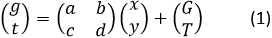
Here, a-d are the constants that dictate the stretching and rotation to get from one co-ordinate system to the other, whilst G and T are the latitude and longitude of the x = y = 0 location on the map.  The task is to adjust all six of these parameters to the values that produce the smallest error when you plug in the x and y co-ordinates of each of your data points and calculate the longitude and latitude, or vice versa.  You could try to adjust all six of these in a single computerized fitting routine to find the best values, but that would require writing your own computer code specific to this particular regression analysis and may well not work anyway.  Adjusting six different parameters all at once to try to find the best values would be like wandering around blindfolded trying to find the highest peak in a mountain range, in six-dimensional space; a difficult task for a computer program or a human.

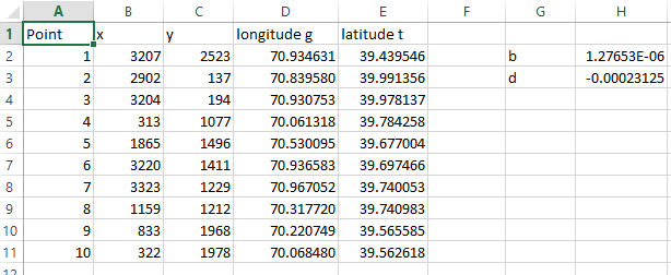
But it is possible to break the problem down into a succession of linear fits, each of which is a simple routine which can be performed on a number of proprietary software packages (I used magicplot).  You begin by obtaining approximate values for 2 of the variables in the rotation / stretching matrix (I chose b and d) using the data from 3 of the data points.  This is just a matter of solving the simultaneous equations you get when you multiply out the matrix above as applied to each data point, so I shall skip this step.  You end up with a set of 10 data points (or as many as you had the patience to type in) and values of b and d calculated using the first 3 data points.  Looking something like this:

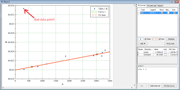
Next, for each (x,y) data point you calculate (g_x,t_x), the values of (g,t) for the location (x,0) (rather than (x,y)).  This is done using the matrix:

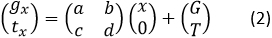
Multiplying out (1) gives separate equations:

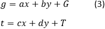
As does multiplying out (2):

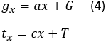
Substituting (4) into (3) gives us:

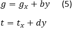
Using the values of b and d from the initial calibration, we can use (5) to calculate g_x and t_x for every data point.  So now we have all our data points in the form:

If we plot graphs of g_x and t_x as a function of x, where each data point is a dot on the graph, they should be reasonably straight lines, described by equation (4) and straight lines can be fitted to them using proprietary software as discussed earlier – this is where the computer does the really hard work for you.  What the computer does is try out lots of different values of a, c, G and T and find the values which result in a straight line passing as close as possible to all the data points.  This is the regression analysis that I mentioned earlier and is the key part of this whole procedure.  This is what allows you to make use of all 10 data points, and weed out the bad ones, rather than just using 3 data points and being a bit stuffed if one of them turns out to be bad.  We can feed in as many data points as we need to, to compensate for the fact that the surveying on google earth is not as accurate as we would like (as discussed earlier).

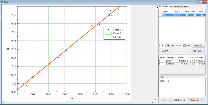
Above is an example of the graph which the computer fits the line to, it has fitted the line and found values for the variables a and G (the variable the computer calls b is actually G).  As you can see, the data points are rather spread out around the fit.  This is because we have used values of b and d which are not that accurate.  Performing the same procedure with the graph of t_x as a function of x gives values for c and T.

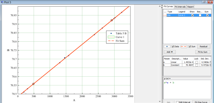
So what we need to do now is use the values of a and C we have just calculated to do more regression analysis to improve our initial guesses at b and d.  To get the set of data points in a suitable form for this we set x = 0, i.e. the following matrix:

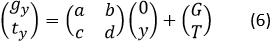
Multiplying out this matrix gives:

Substituting (7) into (3) gives:

Using equation (8) and the values of a and c we have just calculated we can, for each data point calculate (g_y,t_y), the values of (g,t) for the location (0,y).  So we now have all our data points in the form:

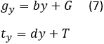
We now plot g_y and t_y as a function of y.  These should also be straight lines (described by equation (7)) and performing the regression analysis gives us more accurate values for b, d, G and T.  We now repeat the first 2 regression analyses with our more accurate values for b, d, G and T.  The second run of the regression analysis I showed in the picture above looked like this:

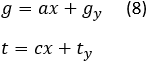
As you can see, the (x,0) data points this time round are lying much closer to the line of best fit.  This is because they have been calculated using the more accurate values of b and d.  The first time round, the computer gave a = 1.4919 x 10^-4.  This time it is saying a = 1.4932 x 10^-4.  To complete the fitting process, i.e. get the most accurate values you can for a, b, c, d, G and T you just repeat the regression analysis in the order described until each analysis gives you the same values as the previous round of regression analysis.  When this is the case you have achieved convergence.  I performed this procedure for several maps covering this area of Kyrgyzstan and needed to do 2 or 3 rounds of regression analysis to achieve convergence – it will take more rounds if one of the data points you used to get the initial values for b and d was a bad one.  There will always be the occasional bad data point – perhaps it was set at a road junction which has been moved since the Soviet map was surveyed, or involves a summit which google earth doesn’t quite have the resolution to get right.  The regression analysis allows you to spot and remove these bad data points – while most data points will lie close to the line of best fit, the bad data point will lie some distance from it.  You can spot this (see example below), delete that data point and rerun the regression analysis without it.

Regression analysis with bad data point

So…we now have accurate values for a, b, c, d, G and T which allow us to take any point on the electronic copy of the Soviet map and, using the pixel co-ordinates (x,y) calculate the latitude and longitude (g,t).  It is sensible at this point to run all our original data points through equation (1) and see how close our calculated latitude and longitude are to what google earth says.  It is also possible to rearrange equation (1) taking the inverse of the a,b,c,d stretching / rotation matrix to get an expression which gives us the pixel co-ordinates (x,y) on the map when we feed in the latitude and longitude (g,t):

Anyway, now we get to the whole point of this exercise, the ability to plot the lines of constant latitude (going roughly but not exactly across the map) and constant longitude (going roughly but not exactly up and down the map).  Each latitude line corresponds to a specific constant value of t.  It starts at a specific value of x (which we decide) near the left-hand side of the map, and finishes at another specific value of x near the right-hand side of the map.  Rearranging equation (3) gives us the value of y which corresponds to each value of x, when we enter t and the other parameters (which we now have accurate values for):

We can also obtain an equation to do the same things for the lines of constant longitude:

Drawing all these lines on the maps takes a while and Phil did most of this…  To finish, here is the section of map shown earlier, with the WGS84 latitude and longitude lines marked on it:

Note that, in the mathematical procedure outlined above, there is nothing to force the latitude and longitude lines to be perpendicular to each other.  They just come out perpendicular to each other anyway, because the procedure is getting them exactly where they should be!  So now, you can read the WGS84 datum latitude and longitude off your GPS (top left corner in the photo below) and locate yourself on the map:

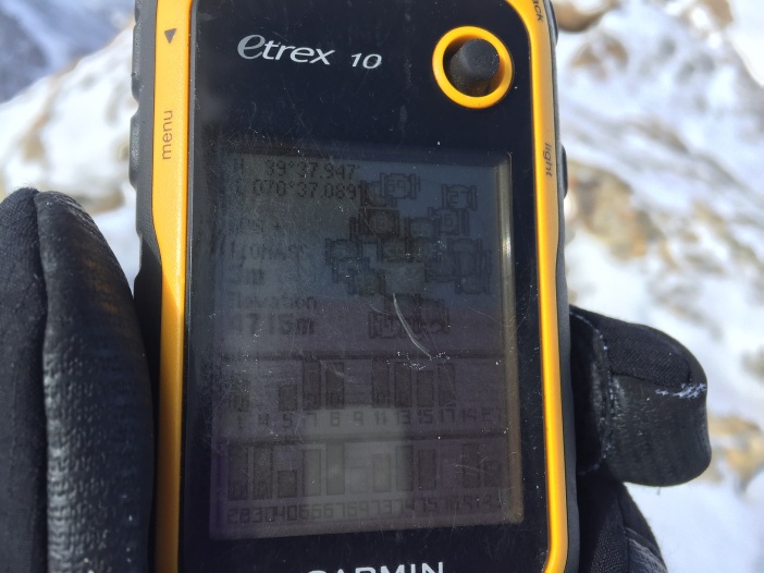
My Garmin etrex 10 GPS, obtained second hand from my good friend and climbing partner Michael Finegan, has seen better days after going on 4 expeditions.  It is getting hard to read the screen (photo copyright (c) Ciaran Mullan).

 

John Proctor

PS I should perhaps mention why it is that I enjoy matrices and regression analysis; in my other life I am a physicist.

 

Our first foray into the mountains

We (Ciaran, John & Phil) finally arrived at basecamp on 5th July, after a longer than expected walk in of two and half days rather than two. Basecamp consisted of a shepherd’s hut, which we used for storing food and cooking when the weather’s bad, along with our two 2-person tents. Ciaran & Phil made their tent setup slightly more palatial by constructing a curved dry stone wall outside and then positioning a tarp betwixt this and the tent porch. It was a claggy day we arrived on, which soon developed into downpours. However, the following morning we were treated to our first proper view of the mountains by a blindly bright white Muz-Tok set against an almost cloudless blue sky.

Morning view from basecamp. Muz-Tok is the peak furthest to the right.

In the afternoon of the 6th, we set off from basecamp with lightweight camping gear towards our first acclimatisation objective; a peak of around 4500-4600m which by our research is unclimbed. We traversed the along the side of the glacier and cut up into one of the smaller valleys towards the peak. After a while of rock hopping, we found a suitably overhanging boulder to call home for night and got settled with the intention of a 4am start the following morning.

Walking in towards the mountains.

Our plans were altered by the arrival of significant snowfall during the night. There was clearly a storm in a nearby valley as the sky was pulsing with a soft white glow as the cloud cover reflected the lightening. The frequency of flashes was impressive, at most about 20 seconds between, from 9pm until 4am non-stop. It was impossible to decipher the direction of the storm, but the absence of thunder was reassuring.

We did encounter an issue with our homely rock. The heat of the day had left the rock (interestingly made of something magnetic, not just granite) warm enough to melt the snow hitting it. The meltwater was then nicely funnelled down the overhang and onto our sleeping bags. Thankfully our bivvy bags were on, but Phil’s was not fully pulled up so his down sleeping bag suffered absolute saturation to the top half.

After an interrupted sleep (to say the least) we had a lazy start in the clearing morning weather. The loose rocky ground was significantly harder to cross now that it had a snow covering, so we aborted the plan to attempt the peak. Instead we opted to walk without gear up the scree for a while to acclimatise. We reached an altitude of 4110m atop a pile of scree before heading back down to basecamp.

John and Phil ascending in the snow.

The pay off for a bad night’s sleep: a glorious morning view of the snow dusted peaks. In the centre is peak Turkestan.

 

Onwards to basecamp…

Anyway, where were we?  It has been that long since we’ve had time to write a post (apologies).  On the road to Batken.  So, to reach our planned basecamp in the Jiptik valley you need to drive from Osh to Batken, then onwards along the road towards Isfara, the very western tip of Kyrgyzstan.  After (arguably) a trip in and out of Tajikistan you turn left off this road and down a rough track for a few hours until you arrive at the village of Sary Zhaz.

Climbers camped at the village of Sary Zhaz.

Sary Zhaz is absolutely the end of the road, but as of this year actually has some visitors.  From Sary Zhaz it is a 2 day hike to the Jiptik valley but the first 1/3^rd of this hike is shared with the approach hike to the Karavshin gorge, which is a (relatively speaking) popular climbing area.  So we shared our campsite at Sary Zhaz with some climbers from the Basque country on their way to the Karavshin.

We were all well fed by locals who have started up a makeshift restaurant to cater for their new visitors. Why is it a new thing that visitors are coming to Sary Zhaz? In the past the approach to the Karavshin involved passing through the politically sensitive Tajik enclave of Vorukh, and the walk-in from Sary Zhaz is, I understand, a new development to cut out that part of the approach.
Our walk-in the next day commenced with a hike uphill from 2,400m to 3,000m; mountains of interest started to come into view – I think this is Pyramidalniy (5,500m).

Pyramidalniy (about 5,500m)

The walk-in to Jiptik involves…well, quite a lot of up and down. We had 6 donkeys, 2 donkey-drivers and another donkey to take our donkey-driver’s stuff. The most extravagant expedition I have ever been on! The whole cavalcade snaked its way down from 3,000m to the crossing over the Karavshin river at 1,600m. Unfortunately Ciaran became ill with a stomach bug (it happens in this part of the world) but we limped on as best we could. At the Karavshin river we had an extended stop in an orchard next to the river, drinking tea whilst eating bread, butter and apricots that we had just picked ourselves from the trees.
The stop was needed as the next stage on the walk-in was an uphill slog from 1,600m to 3,800m – split over late afternoon of this day, and the morning of the following day. We camped at (about) 2,400m. Ciaran and Nurat, one of our donkey-drivers, had to chase a runaway donkey down the hill…. (they donkey lost), and we continued to the mountain pass at 3,800m the next day.

Our donkey train

From the next mountain pass we descended from 3,800m to the Jiptik valley at 2,800m and camped next to the abandoned weather station. The following morning (we were a bit behind schedule) we did the remaining 5 km to our basecamp site and started noticing something that became more and more apparent as we walked further up the valley… Whilst the rock around us was generally limestone (as we expected from the photos we had available), every so often we’d come across a pebble or boulder that looked more like… granite! Much better for climbing on. And it was difficult to see how these granite pebbles and boulders could have come from anywhere other than the mountains at the top of the valley…

A granite pebble surrounded by limestone.

So…what we actually got up to (1)

Now that we are back in the UK, recovered and unpacked (well, nearly) there is a chance to talk about what we got up to.  Myself, Ciaran and Phil arrived in Osh early in the morning on the 30^th June and spent a few days shopping in the bazaar to purchase the food we needed to eat during over 2 weeks on our own in the mountains.  The bazaar is about a mile long and everything under the sun can be purchased there.  On my previous trip (2014) I even found an entire section of the bazaar consisting only of stalls selling cow and goat trotters…. Not joking!

Some views of the Jaima bazaar in Osh

Then it was time to head off into the mountains (2^nd July)…  But there was a hitch.  Robert Taylor’s ship docked at Aberdeen on 30^th June, he was then to take the train to London, fly to Dusseldorf, then on to Moscow, then from Moscow to Osh and arrive early on the 2^nd July to drive with us to the mountains.  However, his flight to Dusseldorf was delayed and he missed his connection to Moscow.  Phil, Ciaran and myself left Osh at 10am on 2^nd July not being sure when (or if) Robert and his baggage would be able to join us.  There was little we could do but arrange for someone from the guesthouse to pick him up from the airport when he did arrive and leave behind directions to the currency exchange office and main stalls in the bazaar.

Anyway…Zhunusbek Karazakov (director of Batken travel service) picked us up from our guesthouse in Osh and we set off on the road to Batken.  For me personally, it was most satisfying that we were now driving off into the least touristy bit of Kyrgyzstan.  The country has seven provinces (oblasts) – Batken, Chui, Jalal-Abad, Naryn, Osh, Talas and Issyk-Kul.  But if you look in a guidebook you can see certain provinces get passed over – Osh province gets 19 pages in the Bradt guidebook and 17 pages in the Odyssey guidebook, whilst poor Batken province gets just 2 pages in the Bradt guidebook and 1 page in the Odyssey guidebook.  The lack of attention received by the region is unfortunate in view of the world-class climbing available there!

Delicious fresh peaches available at the motorway service station on the Osh to Batken road.

We will hopefully post some more next week!

John

Team have arrived in Jiptik valley!

Message from the team via sat-phone: 15:44 on 04/07/16 (BST):

They have arrived at the disused/ruins of the old Weather Station in the remote Jiptik valley, about 5km north from their intended base location.

Whilst they’re running slightly behind schedule, all is well – and they’ve seen some Marco Polo sheep!

---

See their current location on a Big Map!

---

Commentary: Some of the good news is that they’re in – they’re past all the enclaves, borderguards, politics and people – and despite transport kerfuffles, they’re all there and have made it almost to the bottom of the mountain (thanks to their local logistics team from Zhunusbek Karazakov at Batken Travel Service!)

Right now, they’re in a really good location: they’re past the last permanently manned shepherd huts now, and their basecamp is within easy reach. All being well, they should be building camp tomorrow, and be able to start scouting approach routes soon!

We’ll post updates as soon as we get them!

-Tim

Jiptik Weather station (c) Tim Dobson

Making Gear

All this expedition stuff can add up quickly. We are lucky enough to have some great sponsors contributing to our trip (see the “widgets” button at the top for sponsors), but one way I like to save money is by making some of the soft goods I take with me.
Making climbing clothing isn’t going to beat the price of the cheapest stuff in the shops, but if you’re after high quality fabrics anyway it can be significantly cheaper (£30 gore-tex hardshells anyone?). Plus designing it yourself means it’s automatically a tailored fit. In terms of design I like to follow the climbing acronym that Andy Kirkpatrick uses a lot; K.I.S.S. (keep it simple stupid). Less is more for seams in clothing; less possible leaks, less possible thread unravelling, less bulk, etc. And do you really need pockets on every single layer?

Some of the homemade gear coming with me. Clockwise from top left: powerstretch hoody, hi-loft mitts, synthetic insulated gilet, gore-tex pro shell smock, cordura-cotton trousers, ice axe leash, useful heavy duty straps, lightweight crampon bag, fleece pillow (stuffed with a belay jacket)

Having the sewing machine and leftover fabrics from projects is also just useful for repairs and modifications. A while ago I picked up a factory seconds down sleeping bag. It was in phenomenal condition and at a fraction of the price, but unfortunately a women’s size which is just a few inches too short. With scraps of pertex quantum and pertex endurance, along with excess insulation from making a puffy gilet, I made a simple extension around the footbox. It’s had a trial use in the uk, but this expedition will be the thorough test of it and everything else!

The dismembered and reassembled down sleeping bag

Left: my trusty Rab Generator with replacement back panel. Right: Lowe Alpine pack with many pieces replaced (buckles, waist strap, pull cords etc.)

 

Training…

It is now just six days until we fly to Kyrgyzstan, time perhaps to talk a little about the training regime that such an expedition entails.  It is different for all of us; Robert is spending the entirety of June in the middle of the north sea on an oil rig supply vessel so does not really have the option to do running, cycling or climbing.  But at least there is a robust pipe on deck that he can do pullups on when the sea isn’t too rough, and he has been spending an hour a day walking up and down the staircases on the ship carrying a heavy backpack.  Before people feel too sorry for him, he did have the entirety of May off to do trail running and mountain rock climbs.  Robert also knocked off the rather fine sea stack pictured below (Am Buachaille), right at the north-western tip of Scotland, during this month.  Phil and Ciaran are both super-fit anyway so I’m not sure they actually need to do any training.

I, meanwhile, have focussed on weekly trips to the climbing wall and a daily regime of cycling and swimming.  Fortunately I am able to make my commute to work a daily workout as I am now doing an off-road cycle of 11.5 miles to work every morning and then the same again for the return trip in the evening.  My route takes me from my home in north-east Bolton to my workplace in Salford through Moses Gate country park, then up the hill to join the Bury-Manchester cycle route, then through Prestwich forest park and finishing alongside the river Irwell.  It is a relaxing ride speeding along mainly deserted tracks in the woodland and is a better workout than my old on-road cycling route; there are no traffic lights to catch your breath at.

In addition to the cycling I have chucked in a daily swim (750m breaststroke), to work out the muscles I need to hammer those axes into the alpine icefields…  And with all this exercise your weight just drops like a stone if you’re not careful, so I’ve been eating heavily to keep my weight up.  In my experience on expeditions, you typically lose 5-7 kg during the course of the trip so it is best to have a bit in reserve before you set off.  Tuck in to the pasta and the pilaf!

First aid kit

In total we plan to spend 19 days in the mountains – away from roads, mobile internet, medical help, etc. etc…. In the worst case scenario (an accident or injury whilst actually climbing) we could be in a position where it takes an able-bodied person 4 days to get to the nearest road, and another day to a location where medical help may be available. So clearly it is a good idea to take an extensive first aid kit. Here’s (almost all of) what we’re taking this year.

This is the main first aid kit that comes to basecamp.  We take a selection of these items (in smaller quantities) in a camera-sized first aid kit which we carry with us whilst climbing.  Some items in this photo are things we put together for myself and Robert Taylor’s first expedition in 2010, and other things are the result of experience.  Diclofenac is pretty good stuff (painkiller) and doesn’t make you drowsy in our experience, aspirin is good for snow blindness etc.  You need the patience of a saint to use a water filter for every drop of water you use, but if you leave glacial water overnight in a water carrier the sediment will be settled out on the bottom by the morning.

The use of drugs for altitude sickness is a complex and controversial topic on which there are many different opinions.  Some consider that taking drugs such as diamox prophylactically is dangerous, or that it is cheating – like some mountaineering equivalent of an athletic performance-enhancing drug.  My personal view is that it is a bad idea to take drugs for altitude sickness prophylactically, but that it is worth taking small quantities of diamox, dexamethasone and nifedipine in the climbing first aid kit, but only using them in an emergency to permit descent.  In 4 expeditions to altitude I have carried the drugs but never had to take them.  The highest peaks in the area we are visiting are about 5,300m altitude so if you have acclimatized beforehand it should be possible to function without getting altitude sickness.

The first aid kit seems to grow and grow and grow each time I go away to the greater ranges, though partially that is because there are 4 of us this time (the largest expedition I have ever been on!)  Perhaps we will be forced to cut back a bit when we pack and run short of space in our baggage allowance…  When you are staring a potential £200+ bill for excess baggage in the face you have to make some hard decisions.  13 days to go!

Why not Cham?

I’ve had good and bad seasons in Chamonix. In a good season the snow is crisp and firm, the rocks frozen in place, the valleys hot and filled with ice cream vendors. You tick route after route and eat ungodly amounts of food.

A bad season is a very different thing. Snow turns to slush, the rimayes gape open as if to swallow a bus, it chucks down rain till you get trench foot and you start phoning easyjet, begging them to just let it end, checking your bank account to see if you can afford the difference in fares.

Despite the mixed results I’ve had I’ve always enjoyed going to Chamonix. The routes are known all over the world and not just thanks to Gaston; they are things of beauty in their own right, works of art even when separated from the purple prose of ‘The Hundred Finest’. Even in the rain there are burgers to be scoffed and plans to be made. It must stop raining, some time…

Then there is a break in the clouds and you slog up to a hut. The next day dawns bright and crisp, finding you already half way to the summit. Like mist vanishing in the sun, the memories of days reading in your tent to the steady thrum of the rain are gone, replaced with sun drenched summits and the feeling of being high…your lungs turned into a sensory organ, the light unfiltered and clear.

Why, then, would anyone choose to go to Kyrgyzstan instead?

The answer is simple; adventure. Chamonix allows instant access to the mountains via a network of cablecars. While this is great for easy access to the mountains, it does detract from the experience in a way that I didn’t appreciate for a long time. Topping out to have to wade through a sea of selfie-taking tourists is a novelty once but it’s a novelty that soon wears off. The routes are known, described, quantified, graded. One could choose not to read the guidebook, not to look online for beta but really…that would be a bit daft. There are better ways to get a fix of uncertainty.

John, Adam Russell and I went to Kyrgyzstan in 2011 and had a great trip. The travel, the approach, the unknown around every corner…it was something I hadn’t experienced at the time and it influenced what I want climbing to be. That trip delivered adventure in spades but the routes were nowhere near as technical as what I knew I could do, I had done, in the European alps. I was ready for adventure or difficulty; not both.

 

A few more years passed, a few more trips to Chamonix, a trip to Zermatt, more Scottish winter, more rock routes, a steady progression from struggling up voi normales, arriving at the hut long after dark to halving guidebook time, moving quickly and safely in the mountains. A couple of dumb solos, too, before I understood how glaciers can swallow a man whole and realised that was a dumb risk to take. Then, one day, the realisation that the telepherique show is well and good but that it’s time to inject a little exploration again.

Along with Phil and Ciaran (whom I got to know last season in the alps when we shared a campsite) John and I are going to have a bash at combining the sporting and the exploratory. Fast and light is well and good in the alps but this trip will be a case of ‘Strong, Fit and Well Equipped’. Succeed or fail, so long as we come away with the same number of digits we all went with and ideally a few more memories, it’s going to be agood trip.

Plus, I’m off to the Dollies in September so I’m sure I will get my fill of sport then 🙂